Data Analysis
| Descriptive/Qualitative | Statistical/Quantitative |
|---|---|
| -summarize information | -investigate patterns/correlation |
| -make some part of the information easier to understand | -get a measurement of how much data sets differ |
| -visualization | -compute mean values |
| -selection of numbers | -evaluate how appropriate models are/how well a hypothesis fits the data |
Example: Election
Data set: {(Name, given name, ID/PESEL, voted party)}
Entries look like: {(Smith, John, 125634, A),(Mustermann, Max, 04124, B),(Kowalski, Jan, 2137, B),...}
Summary:
1.352.689 votes for party A
2.987.132 votes for party B
522.799 votes for party C
22.911 invalid votes
1.222.572 abstained from voting
Example: Election
Visualization:
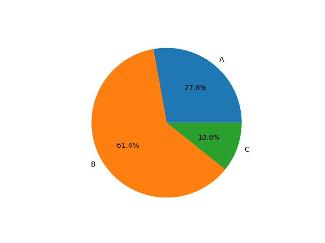
Example: Election
$\Rightarrow$ Party B has majority but not $\frac{2}{3}$.
Problem: Does not explain why people voted like this. Does not explain who voted for whom.
Statistical Data Analysis
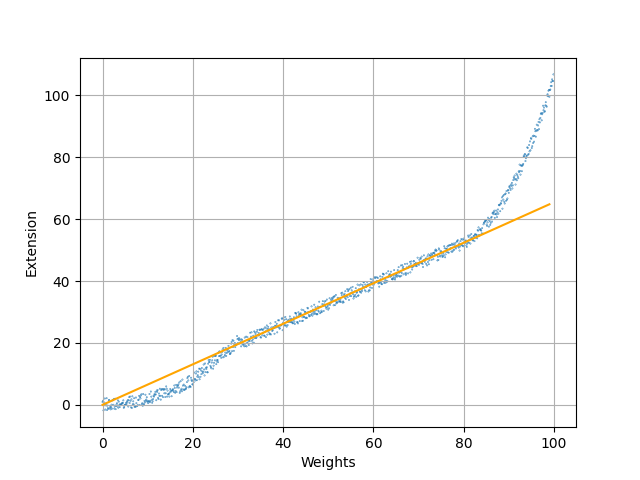
Example from physics: Look at a spring that has some weight attached to it.
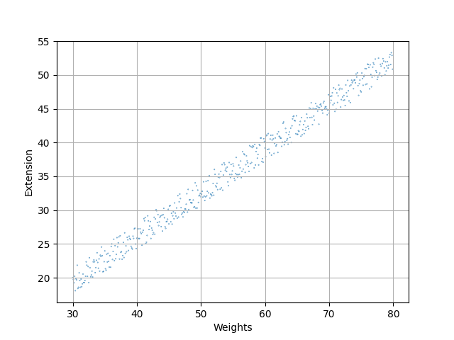
Assumes that the data is given by a linear equation: $\hat{y}=ax+b$
Want to choose line such that distance to data points is minimized, i.e. assume that the deviation from this line is minimal and homogenous.
better: absolute or squared error
Formula for optimal estimates for least square regression:
$$ a= \frac{\frac{1}{n}\sum_{i=1}^n(x_i-\bar{x})(y(x_i)-\bar{y})}{\frac{1}{n}\sum_{i=1}^n(x_i-\bar{x})^2} $$$$ b=\bar{y}-a\cdot \bar{x} $$Linear regression
Example from physics: Look at a spring that has some weight attached to it.
Assume we have the dataset given as two arrazs called "weights" and "extensions":
size = np.array([])
for x in weights:
    size = np.concatenate((size,[0.1]))
plt.scatter(weights,extensions,s=size)
plt.xlabel("Weights")
plt.ylabel("Extension")
plt.grid(True)
coef = np.polyfit(weights,extensions,1)
poly = np.poly1d(coef)
plt.plot(poly(range(0,100)),color='orange')
plt.show()

Obtain empirical Hooke's law: $F=k \cdot x$.
Allows to make predictions, Allows to focus on parameter $k$ to find better explanation.
Linear regression
Example from physics: Look at a spring that has some weight attached to it.
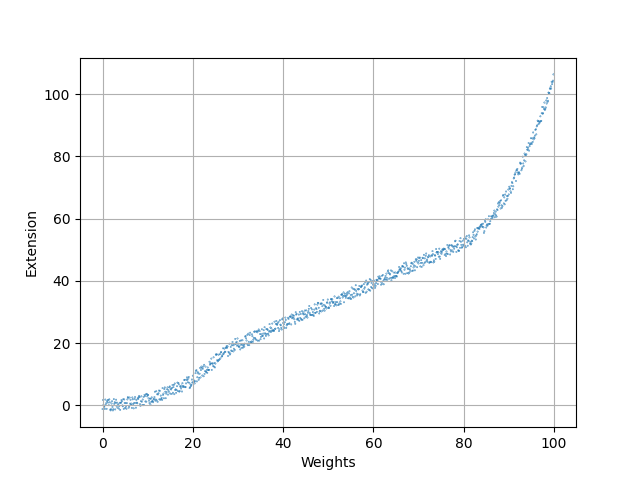
Problem: The model only fits the data for a certain range!
Linear regression
Example from physics: Look at a spring that has some weight attached to it.
Problem: The model only fits the data for a certain range!
$\Rightarrow$ Empirical laws are only valid for the circumstances in which they were found. Be careful with predictions!
Mathematical/Statistical models
What is a model actually?
A model contains:
-a mathematical description of a phenomenon/observation/...
e.g. (linear/polynomial/differentiable/differential) equations, parameters, and variables.
-assumptions and constraints under which the model is supposed to be accurate
In the example: linear model (i.e. linear equation)
parameter: spring constant
variable: weight/force
predicted quantity: string expansion
constraints: only holds in the "elastic range"
Advantages of models
-efficient computation/empirical determination of coefficients and parameters for linear models
-provide precise predictions
-accuracy can be easily checked using statistics
Disadvantages of models
-models are not flexible
-a priori, no way of knowing which model might be accurate
-fitting models is prone to combinatorial explosion if they have too many parameters/coefficients.
Comparing data sets
Once we have choses a model or a statistic, we want to know how well it describes our data set and how it helps us to distinguish different data sets.
Two approaches: Inference vs. Frequency based
Inference: Want to be able to evaluate whether the statistic observed indicates an actual difference or may be a result of some probability distribution.
$\rightarrow$ test a nullhypothesis and decide whether to accept or reject it.
Frequency: Compare relative number of occurences of events in order to see if there is a possible overlap of statistics or not.
$\rightarrow$ compute confidence intervals and discuss if/how much they overlap.
Basics from probability theory
Definition:
A probability space is a triple $(\Omega,\mathcal{F},P)$ with a set of outcomes $\Omega$, a collection of events $\mathcal{F}$ and a probability measure $P$.
A random variable is a measurable function $X: \Omega \rightarrow E$, where $E$ is a measure space.
A probability distribution is the pushforward measure of $P$ on $E$ induced by $X$.
Often: $E=\mathbb{R}$ or $\mathbb{R}^n$.
A probability mass/density function is a function $f: E \rightarrow \mathbb{R}$ such that the probability distribution is given by the sum/integral of $f$.
Hypothesis testing
- Pick a (1-dim) statistic that describes your data set, e.g. mean value, median, slope of regression line, etc.
- Set up null hypothesis $H_0$: the two data sets are sampled from the same distribution
- Specify the random process that is supposed to have created the data, i.e. specify a conjectured probability distribution in detail, called the null distribution
- Compute the probability that, assuming the null hypothesis is true, the difference in the chosen statistic is at least as extreme as the measured one:
This is called the p-value.
- If the observed statistic is too unlikely, we reject the null hypothesis and say that the difference is statistically significant. Common practice: reject if $p<0.05$
Warning: The p-value is not the probability that the null hypothesis is true. The data must come from a random process in order for the p-value to be relevant. The p-value always relies on assumptions on how your data was created $\Rightarrow$ always consider how exactly the specific measurements were made. Also, always report the p-value and not only whether it is above or below 0.05!
Expectation, variance and covariance
Let $X$ be a random variable. Its expected value $E(X)$ is defined as $$ E(X)=\sum\limits_{i=1}^\infty x_i \cdot P(x_i) $$ for $X$ discrete and as $$ E(X) = \int\limits_{-\infty}^\infty x \cdot f(x) dx $$ for $X$ continuous.
The variance of $X$ $\operatorname{Var}(X)$ is defined as $$ \operatorname{Var}(X)= E[(X-E(X))^2] $$
Let $X,Y$ be random variables. The covariance of $X$ and $Y$ $\operatorname{cov}(X,Y)$ is defined as $$ \operatorname{cov}(X,Y)=E[(X-E(X))(Y-E(Y))] $$
The normal distribution
Given two parameters $\mu,\sigma^2$, the normal distribution/Gaussian distribution has the probability density function
$$ f(x) = \frac{1}{\sqrt{2 \pi \sigma^2}}e^{-\frac{(x-\mu)^2}{2\sigma^2}} $$
By Inductiveload - Own work (Original text: self-made, Mathematica, Inkscape), Public Domain, https://commons.wikimedia.org/w/index.php?curid=3817954
Confidence intervals
Basic idea: based on the data, find an interval $(V_1,V_2)$ such that for a parameter $\theta$ we are trying to estimate, the probability $P(V_1\leq \theta \leq V_2)$ has a certain prescribed value usually $P(V_1\leq \theta \leq V_2)=0.95$.
One approach: Central Limit Theorem:
Let $\{X_1,\dots, X_n \}$ be a sequence of indipendent identically distributed random variables, having a distribution with expected value $\mu$ and finite variance $\sigma^2$ and denote the sample average by $$\bar{X}_n = \frac{\sum\limits_{i=1}^n X_i}{n}.$$
Then the random variable $\sqrt{n}(\bar{X}_n-\mu)$ converges to a normal distribution with expected value $0$ and variance $\sigma^2$.
Confidence intervals
$\Rightarrow$ if the sample size is "big enough", we can compute the confidence interval assuming a normal distribution:
Estimate true value by sample mean $\bar{x}_n$, variance given by sample variance: $\frac{\sigma^2}{n}$ (estimated via $\sigma^2 = \sum_{i=1}^n(x_i-\bar{x})^2)$.
Then we have $$P(\bar{X}-\frac{1.96 \sigma}{\sqrt{n}} \leq \mu \leq \bar{X}+\frac{1.96 \sigma}{\sqrt{n}})=0.95 $$ because $\bar{x}-\frac{1.96 \sigma}{\sqrt{n}}$ is the 0.025 quantile and $\bar{x}+\frac{1.96 \sigma}{\sqrt{n}}$ is the 0.975 quantile, i.e. 95% of the measured values lie between them.
$\Rightarrow$ Having computed that for two data sets, we can discuss how much their confidence intervals overlap in order to discuss how likely it is that they are different.
Limits of models
Linear regression revisited
Can also use linear regression in higher-dimensional setting.
Problem: Sometimes some of the variables/parameters may be highly correlated or even linearly dependent!
Definition Let $X,Y$ be random variables. Their correlation coefficient $\operatorname{corr}(X,Y)$ is defined as $$ \operatorname{corr}(X,Y)=\frac{\operatorname{cov}(X,Y)}{\sqrt{\operatorname{Var}(X)\operatorname{Var}(Y)}} $$
$\rightarrow$ there may not exist a unique solution to estimating the parameters but rather a space of solutions. Due to measurement error, one solution from this space is picked but it might not be the ideal one.
One way to adress this: ridge regression
slightly modify the estimator by adding an additional term: instead of minimizing
$$ \lvert \lvert Y-X \alpha \rvert \rvert $$we minimize
$$ \lvert \lvert Y-X \alpha \rvert \rvert + \lambda \lvert \lvert \alpha \rvert \rvert $$More about this in the exercises!
Same mean, same standard deviation, same regression line
Clustering
Classification technique: want to group collections of points together that are not significantly different from one-another.
Hard clustering (actual partition) vs soft clustering (points belong to a cluster with a certain probability)
Usually intermediate step of further analysis
Clustering techniques we want to focus on
-hierarchial clustering (in particular single-linkage)
-centroid based clustering (in particular k-means)
-density based clustering (in particular DBSCAN)
-classification based (in particular k-nearest-neighbors)
Hierarchial clustering:
Want to organize the data points in a hierarchy of clusters. $\rightarrow$ obersve clusters on different scales.
Two basic approaches:
-Agglomerative (bottom-up) - start with one-point clusters and iteratively join clusters with minimal distance
-Divisive (top-down) - start with one cluster and divide according to maximal distance between clusters
Usually agglomerative approach is preferred due to better runtime (naive $\mathcal{O}(n^3)$/optimized $\mathcal{O}(n^2 log(n))$ versus $\mathcal{O}(2^n)$ for divisive).
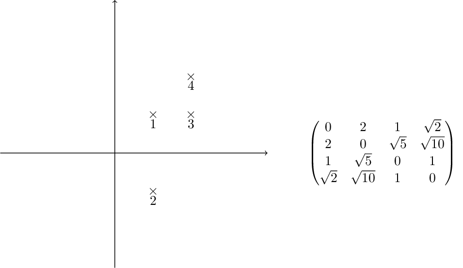
Single linkage clustering
Assume data is given as a distance matrix $D$. We define a sequence of clusters, where each cluster $c$ has a (hierarchial) level $f(c)$.
1: begin with clusters of size 1, all of them of level $f(c)=0$, set iteration number to $m=0$.
2: find the pair of clusters $c_i,c_j$ with minimal distance $D_{ij}$ among all inclusion-maximal clusters with level $<m$.
3: Increment itereation number $m=m+1$. Then merge $c_i\cup c_j$, set $f(c_i\cup c_j)=m$
4: Update the distance matrix by removing the the columns corresponding to $c_i$ and $c_j$ and adding a new row and column for $c_i\cup c_j$ by the formula $d(c_i,c_j)= \operatorname{min}_{a\in c_i, b \in c_j}d(a,b)$.
5: If All points belong to one cluster, return the clustering. Else, continue with step 2.
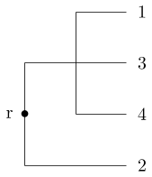
Single linkage clustering
Centroid based clustering
Try to find landmark points $\lambda_i$ (not necessarily part of the data set) such that the clusters are defined by assigning each data point to its closest landmark point.
Problem: How to find the landmark points? How many should it be?
One solution: $k$-means clustering - creates $k$ clusters of points that are centered around $k$ landmark points
1: randomly pick $k$ landmark points $\lambda_1,\dots,\lambda_k$
2: compute the the clusters $c_1,\dots,c_k$ by assigning each data point to its closest landmark point
3: Compute new landmark points $\lambda_i$ given by the center points, i.e. mean value wrt all coordinates, of the clusters $c_i$.
Alternate between 2 and 3 until you are happy with the clusters.
Fact: The within cluster sum of squares decreases monotonously with this process.
$\Rightarrow$ $k$-means clustering converges to a locally optimal clusterin. (Whether it is globally optimal depends on initial random choice of landmark points.)
$k$-means clustering
By Chire - Own work, CC BY-SA 4.0, https://commons.wikimedia.org/w/index.php?curid=59409335
Density-Based Spatial Clustering of Applications with Noise
General idea: seperate data set in three categories depending on the two parameters $\epsilon$ and minPts:
Core points: there are at least minPts points in within distance $\epsilon$ Boundary points: they are not core points but lie in at most distance $\epsilon$ of a core point Outliers: They are more than $\epsilon$ away from any core point
The clustering is created as follows:
- Identify the number of points within distance $\epsilon$ of each data point $\rightarrow$ identify core points
- Say a point $q$ is directly reachable from a core point $p$ if $d(p,q)<\epsilon$. Assing core points that can be reached from another to the same cluster.
- Add boundary points to a cluster from which they can be reached.
- Declare the remaining points to be outliers.

minPts=4
By Chire - Own work, CC BY-SA 3.0, https://commons.wikimedia.org/w/index.php?curid=17045963

By Chire - Own work, CC BY-SA 3.0, https://commons.wikimedia.org/w/index.php?curid=17085332
$k$-nearest-neighbors algorithm
Rough idea: assign a certain feature to data points depending on the feature value of their $k$ nearest neighbors
By Paolo Bonfini - Own work, CC BY-SA 4.0, https://commons.wikimedia.org/w/index.php?curid=150465667
$k$-nearest-neighbors algorithm
For clustering: choose the sum of squares among the $k$ nearest neighbors as the feature and choose the clustering with the smallest overall sum of those. $\rightarrow$ create clusters of $k$ points with minimal sum of cluster sums of squares.
Can also obtain soft/fuzzy clusterings this way by allowing weighted overlap.
Silhouette analysis
How can we decide whether a clustering is "good"?
One option: Silhouette analysis:
Let $C_I$ be a cluster and let $i\in C_I$ be one of its data points. Then we define:
$$ a(i)= \frac{1}{\lvert C_I \rvert -1} \sum\limits_{j\in C_I,j\neq i} d(i,j) $$and $$ b(i)= \min\limits_{J\neq I} \frac{1}{\lvert C_J\rvert} \sum\limits_{j\in C_J} d(i,j) $$ where $C_J$ is any other cluster.
Moreover, we define the silhouette coefficient
$$ s(i)=\frac{b(i)-a(i)}{\max\{a(i),b(i)\}} $$if $\lvert C_I \rvert >1$ and $s(i)=0$ else.
We have $-1<s(i)< 1$. The bigger the value $s(i)$, the more appropriate it is to assign $i$ to $C_I$.
Dimension reduction
Problem: ambient dimension of dataset is very high
Manifold hypothesis: dataset lies on a lower dimensional submanifold.
Question: How to find this submanifold?
General paradigms: feature selection and feature extraction
-Feature selection: want to select a subset for features (i.e. variables and predicted quantities) in order to remove redundant and irrelevant features.
-Feature extraction: combine several features into one in order to reduce the number of features while minimizing information loss
Three techniques we want to look into further
-Principal Component Analysis (PCA)
-t-distributed stochastic neighborhood embedding (t-sne)
-Uniform manifold approximation and projection (UMAP)
(Thank you to Davide Gurnari for his slides on the subject!)
Principal Component Analysis
PCA is a linear dimensionality reduction technique that finds the axes (aka "principal components") along which the variance in the data is maximized.
It then projects data onto these principal components to reduce dimensionality while retaining as much of the original variability as possible.
Let $\mathbf X$ be a $n \times p$ (centered) data matrix.
The covariance matrix is given by $\mathbf C = X^\top \mathbf X/(n-1)$ (Actually this is abuse of notation, but $ X^\top \mathbf X/(n-1)$ is proportional to the actual covariance matrix).
It is a symmetric matrix and so it can be diagonalized: $$ C = V L V^\top,$$ where $ V$ is a matrix of eigenvectors (each column is an eigenvector) and $ L$ is a diagonal matrix with eigenvalues $\lambda_i$ in the decreasing order on the diagonal.
The eigenvectors are called principal axes or principal directions of the data.
The $j$-th principal component is given by $j$-th column of $ {XV}$. The coordinates of the $i$-th data point in the new PC space are given by the $i$-th row of ${XV}$.
SVD and PCA
The singular value decomposition (SVD) of $\mathbf X$ is
$$\mathbf X = \mathbf U \mathbf S \mathbf V^\top$$where $\mathbf U$ is a unitary matrix (with columns called left singular vectors), $\mathbf S$ is the diagonal matrix of singular values $s_i$ and $\mathbf V$ columns are called right singular vectors.
Therefore $$\mathbf C = \mathbf V \mathbf S \mathbf U^\top \mathbf U \mathbf S \mathbf V^\top /(n-1) = \mathbf V \frac{\mathbf S^2}{n-1}\mathbf V^\top,$$ right singular vectors $\mathbf V$ are principal directions (eigenvectors) and that singular values are related to the eigenvalues of covariance matrix via $\lambda_i = s_i^2/(n-1)$.
Principal components are given by $\mathbf X \mathbf V = \mathbf U \mathbf S \mathbf V^\top \mathbf V = \mathbf U \mathbf S$.
Example: Digits
print(X.shape)
fig_digits
(1083, 64)

Source: Scikitlearn
fig, ax = plt.subplots(figsize=(5,4))
plot_embedding(PCA(n_components=2).fit_transform(X, y), 'PCA', ax)

t-Distributed Stochastic Neighbor Embedding
t-SNE minimizes the divergence between probability distributions that represent pairwise similarities in high-dimensional and low-dimensional spaces.
1. Compute Pairwise Similarities in High-Dimensional Space
For each point $x_i$, the probability that $x_j$ is a neighbor of $x_i$
$$ p_{j|i} = \frac{\exp(-\|x_i - x_j\|^2 / 2\sigma_i^2)}{\sum_{k \neq i} \exp(-\|x_i - x_k\|^2 / 2\sigma_i^2)} $$The variance $\sigma_i$ is adapted to the density of the data: smaller values of $\sigma _{i}$ are used in denser regions.
The joint probability $p_{ij}$ is then computed as:
$$ p_{ij} = \frac{p_{j|i} + p_{i|j}}{2N} $$2. Compute Pairwise Similarities in Low-Dimensional Space
In the low-dimensional space, the similarity between pair of points is defined via a Student’s t-distribution with one degree of freedom:
$$ q_{ij} = \frac{(1 + \|y_i - y_j\|^2)^{-1}}{\sum_{k \neq l} (1 + \|y_k - y_l\|^2)^{-1}} $$The t-distribution has heavier tails than a Gaussian. Less similar pairs are penalized less heavily on the lower-dimensional embedding.
3. Minimize the Kullback-Leibler Divergence
t-SNE minimizes the difference between the high-dimensional probability distribution $p_{ij}$ and the low-dimensional distribution $q_{ij}$ using Kullback-Leibler (KL) divergence:
$$ C = \sum_{i \neq j} p_{ij} \log \frac{p_{ij}}{q_{ij}} $$Hyperparameters
The $\sigma_i$ are directly related to perplexity, which controls how many "neighbors" each point considers when measuring similarity.
The relationship between $\sigma_i$ and perplexity is established through an iterative process to find the right $\sigma_i$ for each data point that matches the target perplexity.
What is Perplexity?
Perplexity can be thought of as a smooth measure of the number of nearest neighbors considered for each point. It balances between local structure (small perplexity) and global structure (large perplexity).
The perplexity is defined as:
$$ \text{Perplexity} = 2^{H(P_i)} $$Where $ H(P_i) $ is the Shannon entropy of the conditional probability distribution $P_i$:
$$ H(P_i) = - \sum_j p_{j|i} \log_2 p_{j|i} $$Relationship between $\sigma_i$ and Perplexity:
For each data point $x_i$, t-SNE searches for the value of $\sigma_i$ that makes the entropy $H(P_i)$ approximately equal to the log of the target perplexity:
$$ H(P_i) \approx \log_2(\text{Perplexity}) $$Thus, the correct $\sigma_i$ ensures that the conditional probability distribution $p_{j|i}$ has the desired "spread" of neighbors to match the perplexity.
- Small $\sigma_i$ → Distribution is very narrow → Few neighbors have high probability (low perplexity).
- Large $\sigma_i$ → Distribution is broad → Many neighbors have similar probabilities (high perplexity).
How t-SNE Finds $\sigma_i$:
t-SNE uses binary search on $\sigma_i$ for each data point $x_i$ to ensure the perplexity matches the target value:
- Compute the conditional probabilities $p_{j|i}$ for an initial $\sigma_i$.
- Calculate the entropy $H(P_i)$.
- Adjust $\sigma_i$ using binary search until $H(P_i) \approx \log_2(\text{Perplexity})$.
fig_tSNE

A nice interactive demonstration of t-SNE
https://distill.pub/2016/misread-tsne/
Uniform Manifold Approximation and Projection
UMAP can be used similarly to t-SNE but it claims to capture more of the global structure with superior run time performance.
The algorithm is founded on three assumptions about the data:
- The data is uniformly distributed on a Riemannian manifold;
- The Riemannian metric is locally constant (or can be approximated as such);
- The manifold is locally connected.
Graph Construction in High-Dimensional Space
UMAP first builds a weighted graph in the high-dimensional space:
- k-Nearest Neighbors:
For each data point $ x_i $, UMAP finds its $ k $-nearest neighbors $ \{x_j\} $ using a chosen distance metric.
Fuzzy Graph Representation:
Instead of using fixed edges between points, UMAP uses a fuzzy set to represent local relationships.The edge weight $ w_{ij} $ between two points $ x_i $ and $ x_j $ is given by:
$$ w_{ij} = \exp\left(-\frac{\max(0, d(x_i, x_j) - \rho_i)}{\sigma_i}\right) $$Where:
- $ d(x_i, x_j) $ is the distance between points $ x_i $ and $ x_j $.
- $ \rho_i $ is the distance to the nearest neighbor of $ x_i $, ensuring no zero distances dominate.
- $ \sigma_i $ controls the local scaling and is chosen to balance the neighborhood size.
Optimization in Low-Dimensional Space
In the low-dimensional space, the probability $q_{ij}$ of two points $ y_i $ and $ y_j $ being close is modeled using a Student’s t-distribution.
UMAP tries to minimize the difference between the fuzzy graph in high-dimensional space and the corresponding fuzzy graph in low-dimensional space by minimizingthe following cross-entropy loss:
$$ C = \sum_{i \neq j} w_{ij} \log \left( \frac{w_{ij}}{q_{ij}} \right) + (1 - w_{ij}) \log \left( \frac{1 - w_{ij}}{1 - q_{ij}} \right) $$Hyperparameters
n_neighbors: Controls the size of the local neighborhood used for graph construction.
- Low values → Focuses on fine detail (local structure).
- High values → Focuses on broader patterns (global structure).
min_dist: Controls how tightly UMAP packs points together.
- Low values → Clusters are tighter.
- High values → Clusters are more spread out.
fig_UMAP

Other important concepts from statistics
Questions we want to answer:
Do my chosen features/invariants stay the same if the data set is slightly modified?
$\rightarrow$ stability (under noise)
$\rightarrow$ robustness (under outliers)
How well does my chosen model fit the data?
$\rightarrow$ Goodness of fit tests