Basic idea among all concepts: use a given metric to define a space/simplicial complex as a geometric model (not a statistical model yet!) for the data set
Filtered spaces
Definition:
A filtered space is a sequence of spaces $\{X_t \}_{t \in \mathbb{R}}$ together with embeddings $X_s \hookrightarrow X_t$ for $s < t$.
In fancy language: a functor $X_* : \mathbb{R} \rightarrow (\operatorname{Top},emb)$.
A filtered object in a category $C$, where $C\in \{Top, \ regCW,\ Simp,\ Cub,\ Graph \}$ is a functor $X_* : \mathbb{R} \rightarrow (C,emb)$, where an embedding is understood to be a map that is an isomorphism onto its image.
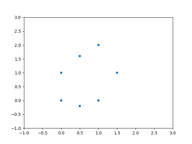
Proximity graphs
The idea is similar to single linkage clustering: inductively add edges of minimal distance. This time, add all such edges.
Definition:
Let $X$ be a point cloud. Its proximity graph of radius $\epsilon$ is defined as $$\operatorname{Pr}(X)_\epsilon := \{(p,q) \vert p,q \in X, d(p,q)\leq \epsilon \}$$
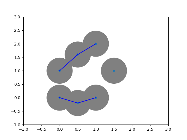
The Vietoris--Rips complex
Named after Leopold Vietoris (introduced parameter dependend homology for metric spaces) and Eliyahu Rips (applied parameter dependend homology to hyperbolic geometry).
Definition: Let $X \subset \mathbb{R}^d$ be a point cloud. The Vietoris--Rips complex of $X$ is defined as $$ \operatorname{VR}_\epsilon(X) := \{\sigma \subset X \vert d(p,q)\leq \epsilon \ \forall p,q \in \sigma \}. $$
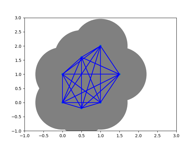
Remark: $\operatorname{VR}_\epsilon(X) \subset \Delta^{\lvert X\rvert -1}$.
$\Rightarrow$ Number of simplices increases exponentially: $2^{\lvert X \rvert}-1$.

VR = gd.RipsComplex(points=points, max_edge_length = 3, )
stree = VR.create_simplex_tree(max_dimension=7)
Complex is of dimension 6 - 127 simplices - 7 vertices. [0] -> 0.00, [1] -> 0.00, [2] -> 0.00, [3] -> 0.00, [4] -> 0.00, [5] -> 0.00, [6] -> 0.00, [0, 4] -> 0.54, [3, 4] -> 0.54, [2, 5] -> 0.64, [1, 5] -> 0.78, [0, 1] -> 1.00, [0, 3] -> 1.00, [0, 3, 4] -> 1.00, [2, 6] -> 1.12, [3, 6] -> 1.12, [5, 6] -> 1.17, [2, 5, 6] -> 1.17, [1, 4] -> 1.30, [0, 1, 4] -> 1.30, [1, 2] -> 1.41, [1, 3] -> 1.41, [0, 1, 3] -> 1.41, [1, 3, 4] -> 1.41, [0, 1, 3, 4] -> 1.41, [1, 2, 5] -> 1.41, [1, 6] -> 1.50, [1, 2, 6] -> 1.50, [1, 3, 6] -> 1.50, [1, 5, 6] -> 1.50, [1, 2, 5, 6] -> 1.50, [4, 6] -> 1.56, [1, 4, 6] -> 1.56, [3, 4, 6] -> 1.56, [1, 3, 4, 6] -> 1.56, [0, 5] -> 1.68, [0, 1, 5] -> 1.68, [3, 5] -> 1.68, [0, 3, 5] -> 1.68, [1, 3, 5] -> 1.68, [0, 1, 3, 5] -> 1.68, [3, 5, 6] -> 1.68, [1, 3, 5, 6] -> 1.68, [4, 5] -> 1.80, [0, 4, 5] -> 1.80, [1, 4, 5] -> 1.80, [0, 1, 4, 5] -> 1.80, [3, 4, 5] -> 1.80, [0, 3, 4, 5] -> 1.80, [1, 3, 4, 5] -> 1.80, [0, 1, 3, 4, 5] -> 1.80, [4, 5, 6] -> 1.80, [1, 4, 5, 6] -> 1.80, [3, 4, 5, 6] -> 1.80, [1, 3, 4, 5, 6] -> 1.80, [0, 6] -> 1.80, [0, 1, 6] -> 1.80, [0, 3, 6] -> 1.80, [0, 1, 3, 6] -> 1.80, [0, 4, 6] -> 1.80, [0, 1, 4, 6] -> 1.80, [0, 3, 4, 6] -> 1.80, [0, 1, 3, 4, 6] -> 1.80, [0, 5, 6] -> 1.80, [0, 1, 5, 6] -> 1.80, [0, 3, 5, 6] -> 1.80, [0, 1, 3, 5, 6] -> 1.80, [0, 4, 5, 6] -> 1.80, [0, 1, 4, 5, 6] -> 1.80, [0, 3, 4, 5, 6] -> 1.80, [0, 1, 3, 4, 5, 6] -> 1.80, [2, 3] -> 2.00, [1, 2, 3] -> 2.00, [2, 3, 5] -> 2.00, [1, 2, 3, 5] -> 2.00, [2, 3, 6] -> 2.00, [1, 2, 3, 6] -> 2.00, [2, 3, 5, 6] -> 2.00, [1, 2, 3, 5, 6] -> 2.00, [0, 2] -> 2.24, [0, 1, 2] -> 2.24, [0, 2, 3] -> 2.24, [0, 1, 2, 3] -> 2.24, [0, 2, 5] -> 2.24, [0, 1, 2, 5] -> 2.24, [0, 2, 3, 5] -> 2.24, [0, 1, 2, 3, 5] -> 2.24, [0, 2, 6] -> 2.24, [0, 1, 2, 6] -> 2.24, [0, 2, 3, 6] -> 2.24, [0, 1, 2, 3, 6] -> 2.24, [0, 2, 5, 6] -> 2.24, [0, 1, 2, 5, 6] -> 2.24, [0, 2, 3, 5, 6] -> 2.24, [0, 1, 2, 3, 5, 6] -> 2.24, [2, 4] -> 2.26, [0, 2, 4] -> 2.26, [1, 2, 4] -> 2.26, [0, 1, 2, 4] -> 2.26, [2, 3, 4] -> 2.26, [0, 2, 3, 4] -> 2.26, [1, 2, 3, 4] -> 2.26, [0, 1, 2, 3, 4] -> 2.26, [2, 4, 5] -> 2.26, [0, 2, 4, 5] -> 2.26, [1, 2, 4, 5] -> 2.26, [0, 1, 2, 4, 5] -> 2.26, [2, 3, 4, 5] -> 2.26, [0, 2, 3, 4, 5] -> 2.26, [1, 2, 3, 4, 5] -> 2.26, [0, 1, 2, 3, 4, 5] -> 2.26, [2, 4, 6] -> 2.26, [0, 2, 4, 6] -> 2.26, [1, 2, 4, 6] -> 2.26, [0, 1, 2, 4, 6] -> 2.26, [2, 3, 4, 6] -> 2.26, [0, 2, 3, 4, 6] -> 2.26, [1, 2, 3, 4, 6] -> 2.26, [0, 1, 2, 3, 4, 6] -> 2.26, [2, 4, 5, 6] -> 2.26, [0, 2, 4, 5, 6] -> 2.26, [1, 2, 4, 5, 6] -> 2.26, [0, 1, 2, 4, 5, 6] -> 2.26, [2, 3, 4, 5, 6] -> 2.26, [0, 2, 3, 4, 5, 6] -> 2.26, [1, 2, 3, 4, 5, 6] -> 2.26, [0, 1, 2, 3, 4, 5, 6] -> 2.26
The Vietoris--Rips complex
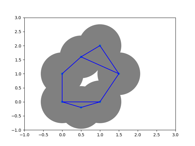
Definition Let $G$ be a graph. A clique in $G$ is a subgraph $G'\subset G$ that is isomorphic to a complete graph. The flag complex/clique complex of $G$ is defined as $$ \operatorname{Cl}(X):= \{\sigma \subset X \vert \sigma \text{ is a clique} \} $$
Observation: The Vietoris--Rips complex is the clique complex of the proximity graph.
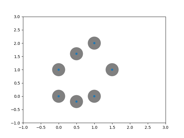
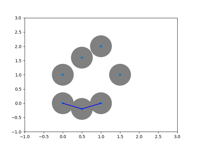
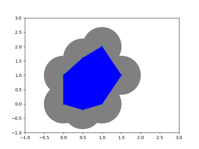
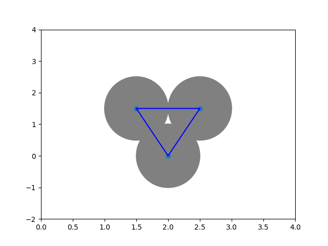
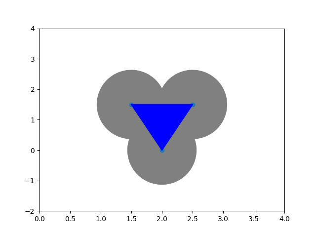
The Čech complex
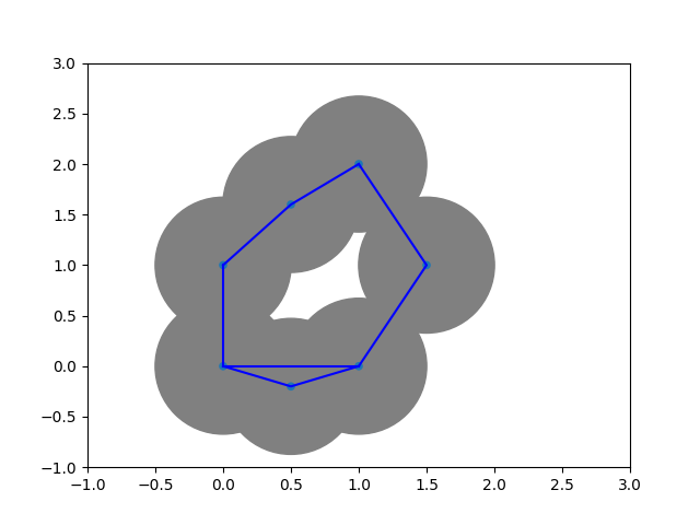
Definition: Let $X$ be a point cloud. The Čech complex of $X$ is defined as
$$ Č_\epsilon(X):=\{\sigma \in X \vert \bigcap_{p\in \sigma} B_\epsilon(\sigma)\neq \emptyset \} $$Definition: Let $X$ be a space and let $\mathcal{U}:=\{U_i\}_{i \in I}$ be a cover of $X$. The nerve of $\mathcal{U}$ is the simplicial complex $\mathcal{N}(\mathcal{U})$ that has
-vertices: $U_i$
-n-simplices: $\{U_{i_0},U_{i_1},\dots,U_{i_n} \}$ such that $\bigcap_{{i_0},{i_1},\dots,{i_n}} U_{ij}$
The Čech complex
Theorem(Nerve Theorem): Let $X\subset \mathbb{R}^n$ be a subspace and let $\mathcal{U}$ be a closed and convex cover of $X$. Then $\mathcal{N}(\mathcal{U})\cong X$.
Remark: Following the manifold hypothesis, there could be an $\epsilon$ such that the intersection of the closed $\epsilon$-balls with the unknown manifold $M$ that the point cloud is sampled from form a closed convex cover of $M$. In that case, the Čech complex recovers the correct homotopy type!
Problem: We do not know the correct $\epsilon$ and we are not able to do the intersection because we do not know $M$. Additionally, for large $\epsilon$ we obtain $\Delta^{\lvert X \rvert -1}$ again.
Observation: The Čech complex is the nerve of the $\epsilon$-balls
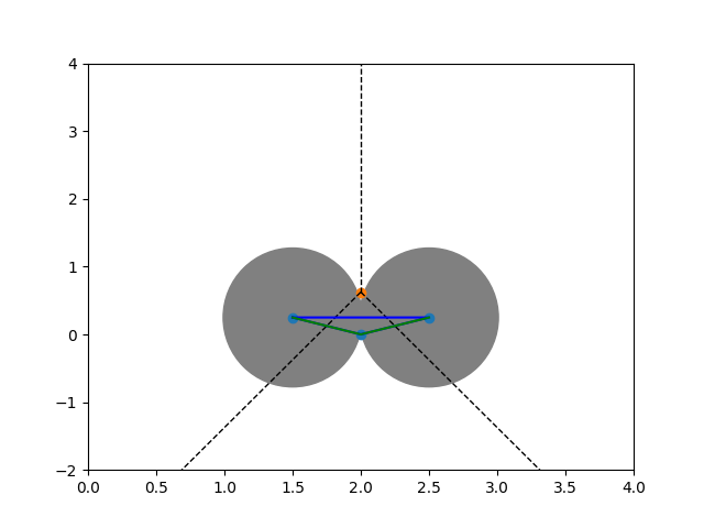
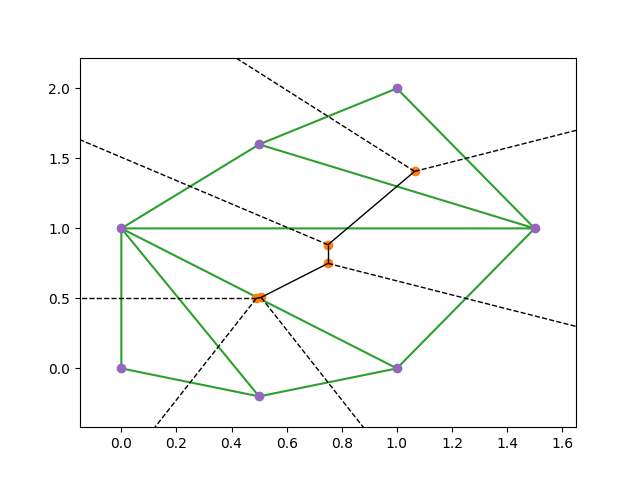
Voronoi cells and the Delaunay triangulation
Problem with Vietoris--Rips and Čech: both are abstract and not embedded in $\mathbb{R}^n$.
Possible solution: Voronoi cells (named after Georgy Voronoi, mathematician of Ukrainian descent, Professor at University of Warsaw)
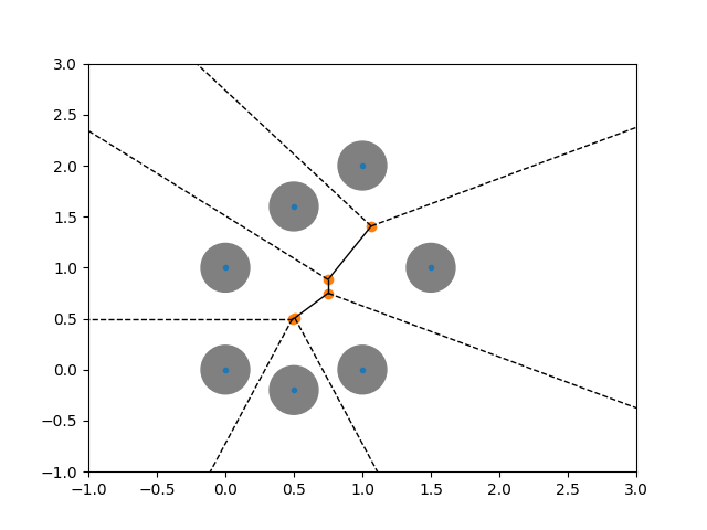
Definition: Let $X\subset \mathbb{R}^n$ be a point cloud and let $p\in X$ be a point. The Voronoi cell of $p$ is defined as
$$ Vor(p,X):=\{q\in \mathbb{R}^n \vert d(p,q)\leq d(p',q) \forall p'\in X\setminus \{p\} \} $$
Vor = Voronoi(points)
fig= voronoi_plot_2d(Vor)
ax = plt.gca()
ax.set_xlim([-1, 3])
ax.set_ylim([-1, 3])
(-1.0, 3.0)

Voronoi cells and the Delaunay triangulation
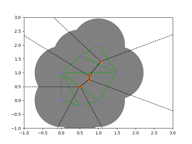
Definition: Let $X\subset \mathbb{R}^n$ be a point cloud. The Voronoi diagram associated with $X$ is the closed convex cover given by the Voronoi cells.
The Delaunay triangulation $\operatorname{Del}(X)$ associated with $X$ is the nerve of the Voronoi diagram.
The Delaunay complex/ Alpha complex
We want to combine both approaches:
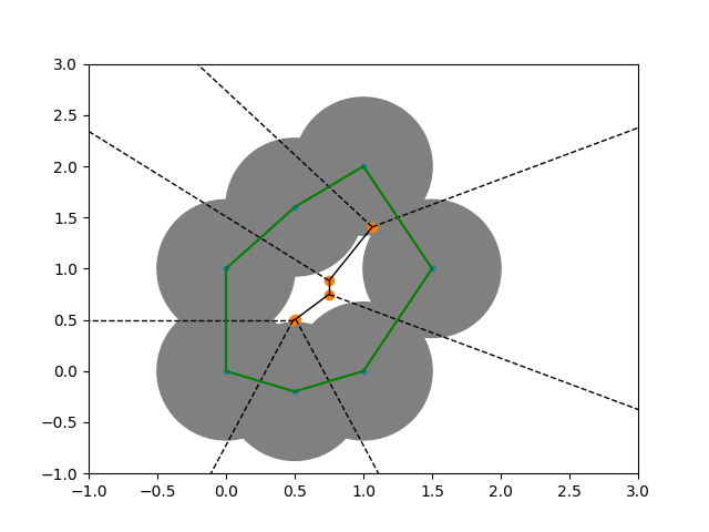
Definition: Let $X\subset \mathbb{R}^n$ be a point cloud and let $p\in X$ be a point. The Voronoi ball of radius $\epsilon$ around $p$ is defined as $$ \operatorname{Vor}_\epsilon(p,X):= B_\epsilon(p) \cap \operatorname{Vor}(p,X). $$
The Delaunay complex $\operatorname{Del}_\epsilon$ of $X$ is the nerve of the Voronoi balls.
The Delaunay--Čech complex
A similar but slightly different approach is the Delaunay--Čech complex:
Definition: Let $X\subset \mathbb{R}^n$ be a point cloud. The Delaunay--Čech complex of $X$ is defined as $$ \operatorname{DelČ}_\epsilon(X) := \{\sigma \in \operatorname{Del}(X) \vert \bigcap_{p\in \sigma} B_{\epsilon}(p)\neq \emptyset \} $$